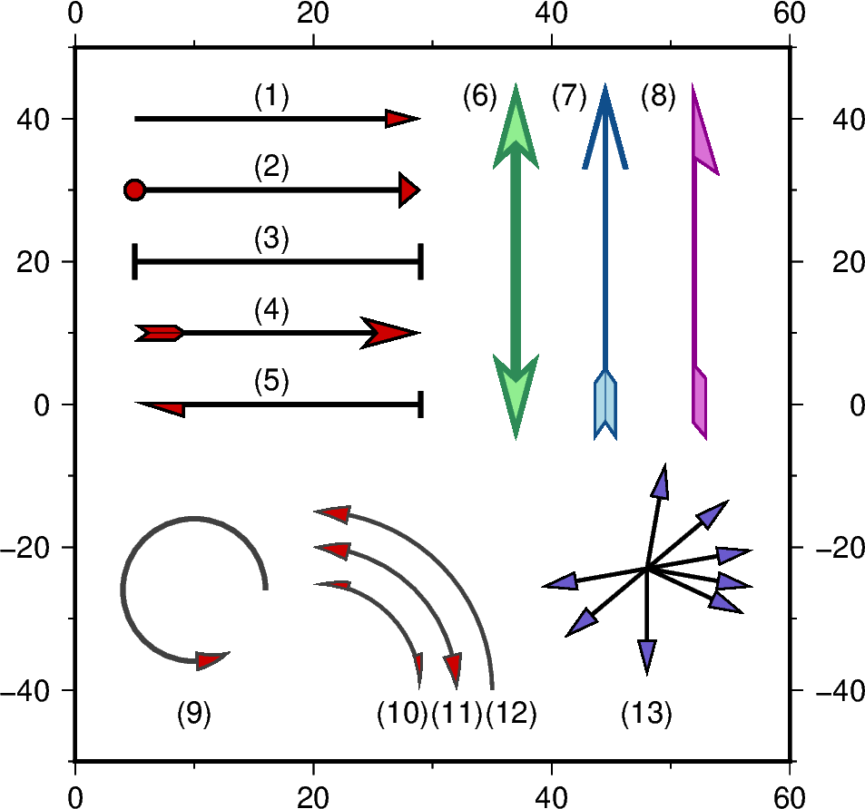
Vectors

The pygmt.Figure.plot method can plot individual types of vectors. There are three classes of vectors: Cartesian, circular and geographic. While their use is slightly different, they all share common modifiers that affect how they are displayed.

The following vectors are available:

• v: vector, x`, y, direction

• m: math arc angle, x`, y, direction

• =: geographic vector, x`, y, direction

Upper-case versions V and M are similar to v and m but expect geographic azimuths and distances.

import numpy as np
import pygmt

fig = pygmt.Figure()
fig.basemap(region=[0, 60, -50, 50], projection="X10c/10c", frame=True)

Plot simple horizontal vectors (1)-(5)

x = 5
y = 40
idx = 1

for vecstyle in [
    "v0.5c+e",  # (1) simple vector with arrow head at the end
    "v0.3c+bc+ea+a80",  # (2) vector with arrow head at the end and a circle at the beginning
    "v0.3c+bt+et+a80",  # (3) vector with terminal lines at beginning and end
    "v0.85c+bi+ea+h0.5",  # (4) vector with tail at the beginning and an arrow with modified vector head at the end
    "v0.7c+bar+et",  # (5) vector with half-sided arrow head at the beginning and terminal line at the end
]:
    fig.plot(x=x, y=y, style=vecstyle, direction=([0], [4]), pen="2p", color="red3")
    fig.text(x=16.5, y=y + 3.5, text="(" + str(idx) + ")")
    y -= 10  # move the next vector down
    idx += 1

Plot simple vertical vectors using different pens and colors (6)-(8)

x = 37
y = -5

vectorsv = [
    ["v1.2c+e+b+h0.5", "lightgreen", "4p,seagreen"],  # (6)
    ["v1.2c+bi+eA+h0.2", "lightblue", "2p,dodgerblue4"],  # (7)
    ["v1.3c+bi+ea+h0.4+r", "orchid", "2p,darkmagenta"],  # (8)
]

for vector in vectorsv:
    fig.plot(
        x=x, y=y, direction=([90], [5]), style=vector[0], color=vector[1], pen=vector[2]
    )

    fig.text(x=x - 3, y=43.5, text="(" + str(idx) + ")")

    x += 7.5
    idx += 1

Plot circular vectors (9)-(12)

# (9) plot a math angle arc with its center at 10/-26,
#     a radius of 1 and a start angle of 0 and end angle of 300 degrees
data = np.array([[10, -26, 1, 0, 300]])
fig.plot(data=data, style="m0.5c+ea", color="red3", pen="2p,gray25")

fig.text(x=10, y=-43, text="(" + str(idx) + ")")
idx += 1

# (10-12) plot math angle arcs starting at 0 degrees and ending at 90 degrees
#         with different radii and start/end vector modifiers
x = 20
y = -40
startdir = 0
stopdir = 90
radius = 1.5
pen = "1.5p,gray25"
xtext = 24.5

for arcstyle in [
    "m0.5c+ea+ba+r",  # (9) right-sided half-arrow heads at beginning and end
    "m0.5c+ea+ba",  # (10) arrow head at beginning and end
    "m0.5c+ea",  # (11) arrow head at the vector end
]:

    data = np.array([[x, y, radius, startdir, stopdir]])
    fig.plot(data=data, style=arcstyle, color="red3", pen=pen)

    fig.text(x=xtext + 3, y=-43, text="(" + str(idx) + ")")

    radius += 0.5
    xtext += 4.55
    idx += 1

Plot set of vectors with arrow ends starting from one center point (13)

x = np.repeat(48, 8)
y = np.repeat(-23, 8)
lengths = np.repeat(1.5, 8)

fig.plot(
    x=x,
    y=y,
    direction=([80, 50, 10, 100, 260, 115, 180, 230], lengths),
    style="V0.5c+e",
    color="slateblue",
    pen="1.5p",
)

fig.text(x=48, y=-43, text="(" + str(idx) + ")")
idx += 1

fig.show()

Out:

<IPython.core.display.Image object>